Introduction to Pandas

[3]:

import pandas as pd
import seaborn as sns
import matplotlib.pyplot as plt
from pprint import pprint

What is a pandas DataFrame

Pandas is a library
- (import it, has a documentation website https://pandas.pydata.org/)
DataFrame is a datatype/datastructure/object
- the main offering of the pandas library

Why use pandas DataFrames

Pandas DataFrame Description/Motivation
- Robust tool for data wrangling and data analysis
- Exceptionally good documentation
- Synergizes with other libraries
- More powerful than excel
Use-case
- In-memory amount of data
- Millions of rows

Clear example of DataFrame

Attributes
- Column Indexes
- Row Indexes
- Multiple datatypes
- Datatypes function of column
  - List of strings in the entry at [4,‘column_three’]

How are they made?

They are declared
The information comes from
- read in a .csv file
- from a python dictionary
- from a pickle (special binary file)
- from .json file
- and more

Making the above DataFrame

Strategy
- DataFrame from a python dictionary (less common, but helpful for now)
If we were unsure
- https://pandas.pydata.org/docs/reference/api/pandas.DataFrame.from_dict.html
We make a dictionary where
- the keys are column names
- the values are lists of actual data

[4]:

#make the values
first_list=[1,2,3,4,5]
second_list=['a','b','c','d','e']
third_list=['lets','mix','it','up',['ok']]

[5]:

#assign the values to keys in a dictionary
my_dict={
    'column_one':first_list,
    'column_two':second_list,
    'column_three':third_list
}

[6]:

#print the whole dictionary to see what it looks like
#note that the keys are ordered alphabetically when we use pprint (pretty print)
pprint(my_dict)

{'column_one': [1, 2, 3, 4, 5],
 'column_three': ['lets', 'mix', 'it', 'up', ['ok']],
 'column_two': ['a', 'b', 'c', 'd', 'e']}

[7]:

#declare our dataframe using the "from dictionary approach"
#get our "information" from our dictionary
my_DataFrame=pd.DataFrame.from_dict(my_dict)

[8]:

#see our dataframe
my_DataFrame

[8]:

	column_one	column_two	column_three
0	1	a	lets
1	2	b	mix
2	3	c	it
3	4	d	up
4	5	e	[ok]

Accessing Values in a DataFrame

Accesing the Indices (indexes)

The indices are accessible and mutable (changeable)

[9]:

print(my_DataFrame.index)

RangeIndex(start=0, stop=5, step=1)

[10]:

print(my_DataFrame.columns)

Index(['column_one', 'column_two', 'column_three'], dtype='object')

Accesing cells by numeric location

Values DataFrames can be accessed “like” traditional lists (according to numerical position).

[11]:

my_DataFrame.iloc[2,1]

[11]:

'c'

This can be a mildly dangerous approach if you are writing for long-term projects. But can be convenient for some quick-scripts.

Accessing cells by index/column-names

“at” is a good choice for single-value access

[12]:

my_DataFrame.at[2,'column_three']

[12]:

'it'

“loc” is a good choice for “slicing” a dataframe (provide a list of row-indices and a list of column-indices)

[13]:

my_DataFrame.loc[0:2,['column_two','column_three']]

[13]:

	column_two	column_three
0	a	lets
1	b	mix
2	c	it

Accessing cells by condition

We can write conditions “inside loc” in order to get slices where the condition is true (fyi: under the hood, python turns the condition into a list of True/False)

[14]:

my_DataFrame.loc[
    my_DataFrame['column_one'] > 2
]

[14]:

	column_one	column_two	column_three
2	3	c	it
3	4	d	up
4	5	e	[ok]

Operations on a DF

We can loosely classify operations on a DF into “simple” and “complicated”. The general strategy for each type of operation is shown below.

Simple Operations

Rule of thumb definition
- If the operation feels “common”, then see (google) if there is a built-in function
Examples
- Taking the average of a column
- Adding a constant to a column
- Stripping the whitespace from the ends of strings in a column
Advice
- Use the built in function.
  - Fast
  - Error-free

[15]:

#taking the average value of a column
#same thing as my_DataFrame['column_one'].mean()
my_DataFrame.column_one.mean()

[15]:

3.0

[16]:

#adding a constant value to a column
my_DataFrame.column_one+5

[16]:

0     6
1     7
2     8
3     9
4    10
Name: column_one, dtype: int64

A Caveat

[17]:

#notice in the above we did not assign the output of "my_DataFrame.column_one+5" to anything.
#so the original dataframe remains unchanged
my_DataFrame

[17]:

	column_one	column_two	column_three
0	1	a	lets
1	2	b	mix
2	3	c	it
3	4	d	up
4	5	e	[ok]

[18]:

#removing the whitespace from a column
my_DataFrame.column_two.str.strip()

[18]:

0    a
1    b
2    c
3    d
4    e
Name: column_two, dtype: object

Notice that we needed to “access” the “string representation” of a column in order to “do an operation” that “acts on strings”. With a little practice you will get used to these things.

More Complicated Operations

Rule of thumb definition
- As the “customness” of an operation increases, so do the chances that you will have to write the operation yourself.
Advice
- If the project does not call for it, do not break your back to force the use of fast functions.
- Instead, consider “operating” “element-wise” “in a for-loop”
Examples
- Each element in a column is searched against a database
- Each list in a column has some complicated math done on it

One approach is iterrows

[30]:

#iterrows gives us two things that we iterate over simultaneously, much like enumerate() on a
#"normal" list
for temporary_index,temporary_row in my_DataFrame.iterrows():
    #COMPLICATED CODE HERE
    #printing example:
    if temporary_index==2:
        print(temporary_index)
        print('*'*30)
        print(temporary_row)
        print('*'*30)
        print(temporary_row['column_two'])

2
******************************
column_one       3
column_two       c
column_three    it
Name: 2, dtype: object
******************************
c

Synergies with other libraries

Getting a larger dataset

[20]:

#the penguins dataset is a "classic"
my_dataset=sns.load_dataset('penguins')

[21]:

my_dataset

[21]:

	species	island	bill_length_mm	bill_depth_mm	flipper_length_mm	body_mass_g	sex
0	Adelie	Torgersen	39.1	18.7	181.0	3750.0	Male
1	Adelie	Torgersen	39.5	17.4	186.0	3800.0	Female
2	Adelie	Torgersen	40.3	18.0	195.0	3250.0	Female
3	Adelie	Torgersen	NaN	NaN	NaN	NaN	NaN
4	Adelie	Torgersen	36.7	19.3	193.0	3450.0	Female
...	...	...	...	...	...	...	...
339	Gentoo	Biscoe	NaN	NaN	NaN	NaN	NaN
340	Gentoo	Biscoe	46.8	14.3	215.0	4850.0	Female
341	Gentoo	Biscoe	50.4	15.7	222.0	5750.0	Male
342	Gentoo	Biscoe	45.2	14.8	212.0	5200.0	Female
343	Gentoo	Biscoe	49.9	16.1	213.0	5400.0	Male

344 rows × 7 columns

Note that we can no longer see every row and every column. This will be especially true in datasets with thousands (of thousands) of rows. We want to be able to interrogate the dataset as a whole.

Basic inspection - Some handy functions

[22]:

my_dataset.info()

<class 'pandas.core.frame.DataFrame'>
RangeIndex: 344 entries, 0 to 343
Data columns (total 7 columns):
 #   Column             Non-Null Count  Dtype
---  ------             --------------  -----
 0   species            344 non-null    object
 1   island             344 non-null    object
 2   bill_length_mm     342 non-null    float64
 3   bill_depth_mm      342 non-null    float64
 4   flipper_length_mm  342 non-null    float64
 5   body_mass_g        342 non-null    float64
 6   sex                333 non-null    object
dtypes: float64(4), object(3)
memory usage: 18.9+ KB

info() shows us
- column names
- non-null counts
- datatypes
- memory usage

[23]:

my_dataset.describe()

[23]:

	bill_length_mm	bill_depth_mm	flipper_length_mm	body_mass_g
count	342.000000	342.000000	342.000000	342.000000
mean	43.921930	17.151170	200.915205	4201.754386
std	5.459584	1.974793	14.061714	801.954536
min	32.100000	13.100000	172.000000	2700.000000
25%	39.225000	15.600000	190.000000	3550.000000
50%	44.450000	17.300000	197.000000	4050.000000
75%	48.500000	18.700000	213.000000	4750.000000
max	59.600000	21.500000	231.000000	6300.000000

describe() gives us some descriptive statistics of numeric columns
- look at these values together (dont assume normality, etc)

Visualizing our Dataset

[24]:

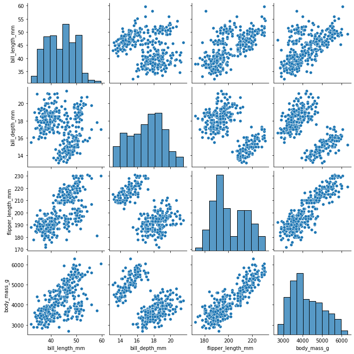
#seaborn's pairplot very conveniently accepts a dataframe as input
#and makes a scatter/histogram figure
sns.pairplot(
    my_dataset
)

[24]:

<seaborn.axisgrid.PairGrid at 0x7fdd79011f40>

[25]:

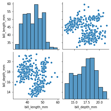
#we could send a smaller dataframe using a list of columns if we wanted
sns.pairplot(
    my_dataset[['bill_length_mm','bill_depth_mm']]
)

[25]:

<seaborn.axisgrid.PairGrid at 0x7fdd79121a00>

[26]:

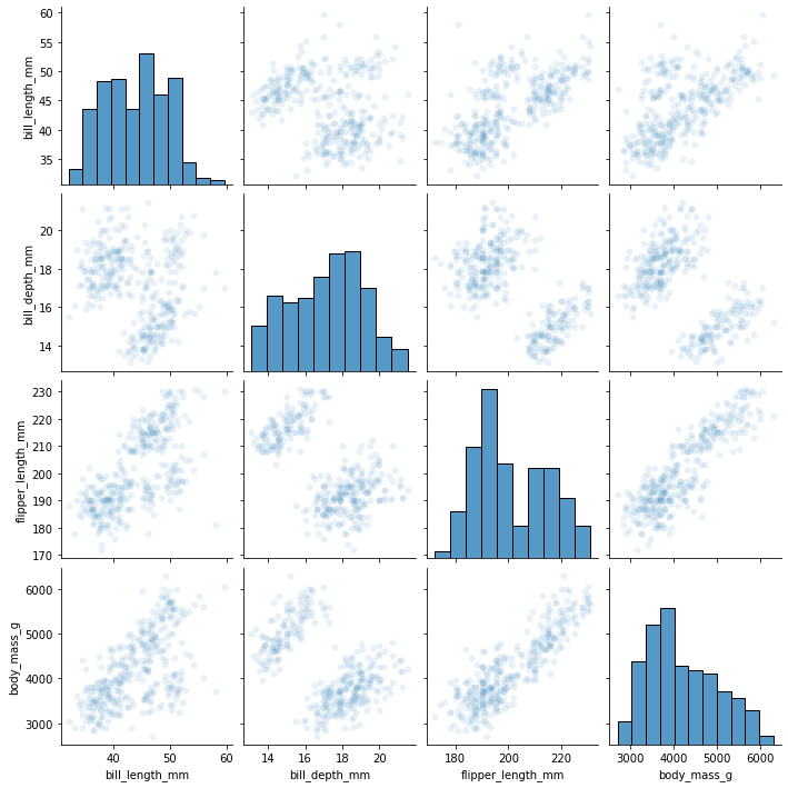
sns.pairplot(
    my_dataset,
    #seaborn is built "on top of matplotlib", which means that it does a lot of things
    #more easily for you
    #however, some of the stuff in matplotlib is still accessible if you can express
    #what you want the same way.
    #if we had millions of datapoints, we could visualize density by making the points
    #somewhat transparent
    plot_kws={'alpha':0.1}
)

[26]:

<seaborn.axisgrid.PairGrid at 0x7fdd7529e1f0>

[27]:

#coloring based on a categorical variable is very natural
sns.pairplot(
    my_dataset,
    hue='species'
)

[27]:

<seaborn.axisgrid.PairGrid at 0x7fdd6f1e9760>

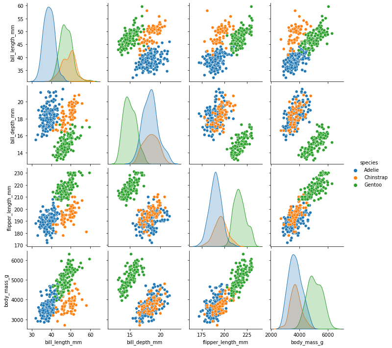
Our histograms have been transformed into (normalized?) densities.

There are way more types of plots where that came from

[28]:

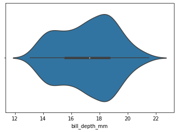
sns.violinplot(
    x=my_dataset.bill_depth_mm
)

[28]:

<AxesSubplot:xlabel='bill_depth_mm'>

[29]:

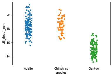
sns.stripplot(
    x='species',
    y='bill_depth_mm',
    data=my_dataset
)

[29]:

<AxesSubplot:xlabel='species', ylabel='bill_depth_mm'>

[ ]:

[ ]:

day_1_file_parsed=pd.read_csv('./Day1CountryInfo2018.txt')